Quantifying Support and Resistance: Proximity-Weighted CBD

Cost basis has long been a cornerstone of on-chain analytics. From cohort-specific realized price bands, often treated as dynamic support and resistance, to indicators like Market Value to Realized Value Ratio (MVRV) and Net Unrealized Profit/Loss (NUPL) that use cost basis to quantify the market’s embedded profit and loss, these tools help investors frame macro tops, bottoms, and regime shifts. Cost Basis Distributions (CBD) build on the same foundation with a more granular lens: instead of reducing the market to a single anchor, they map where supply last changed hands across price levels, revealing the dynamic “inventory structure” that shifts across time.

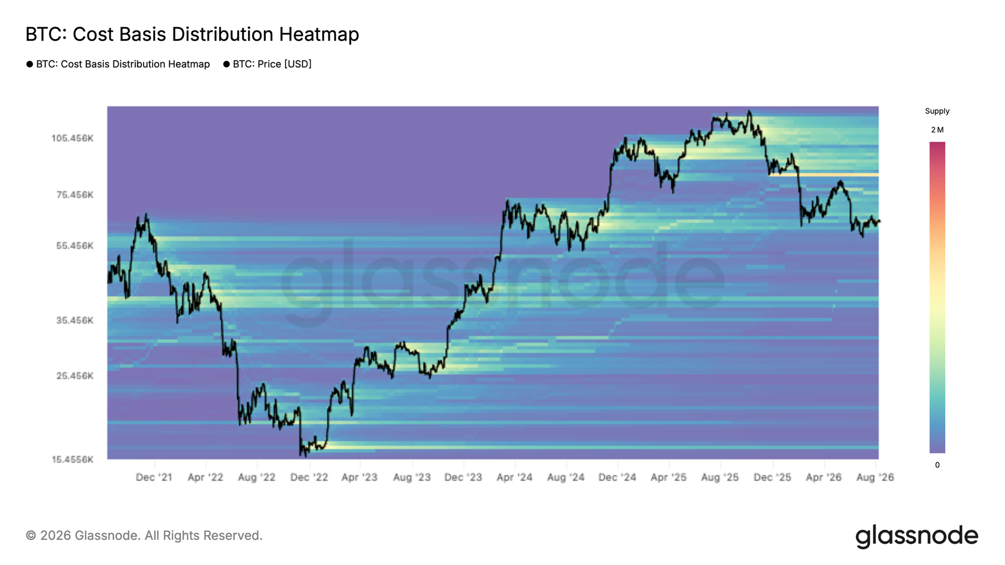
The challenge is that our most common cost-basis metrics, whether market-wide measures or cohort-based indicators, don’t consistently capture where actionable liquidity sits relative to spot. Aggregate indicators are useful regime references, but they’re dominated by the largest, slowest-moving pools of supply and can underweight the nearby clusters that price is about to test. Cohort indicators (e.g., short-term holder metrics) are more reactive and excellent for tracking the most active group’s behavior, but they can miss broader supply “walls”, especially when price is approaching a sizeable cluster held by longer-term investors whose cost basis is near spot. Cost Basis Distributions help close that gap by explicitly showing where supply is concentrated across price levels and, when tracked through time, by making it possible to visualize how that inventory structure evolves as tokens change hands. The trade-off is that this view is inherently high-dimensional, so it’s still most often consumed as a heatmap or qualitative read, informative but difficult to compare day-to-day and hard to integrate systematically into a single, clean time series signal.

Proximity-weighted Cost Basis Distribution tackles these challenges by translating the distribution into a compact time series without losing the practical question that matters most: where is the market’s “tradeable” supply concentrated, and how is it positioned versus the current price?

Proximity Support–Resistance (PSR): Concept & Weighting

Building on the Cost Basis Distribution (CBD) framework, Proximity Support–Resistance (PSR) turns the distribution heatmap into a compact, time-series measure by explicitly weighting supply by its distance to spot. Supply positioned below spot is interpreted as potential support, while supply above spot represents potential overhead resistance. The resulting Proximity Support Index (PSI) is the share of proximity-weighted supply that lies below spot, and the Proximity Resistance Index (PRI) is the complementary share above spot. To keep the signal temporally consistent and comparable across cycles, PSR is computed on Cost-Basis Quantiles (CBQ), a percentile-based representation of CBD.

The specific calculations for PSI and PRI are as follows:

$$\begin{aligned} \text{PSI}_t &= \frac{\text{PS}_t}{\text{PS}_t + \text{PR}_t} \in [0,1] \ \text{PRI}_t &= \frac{\text{PR}_t}{\text{PS}_t + \text{PR}_t} \in [0,1] \end{aligned}$$

where  (proximity support) and  (proximity resistance) are defined by: 

$$\text{PS}_t = \sum_{\varphi=1}^{100} w_{(\varphi,t)} \, \mathbf{1}\{P_t > RP_{(\varphi,t)}\}$$

$$\text{PR}_t = \sum_{\varphi=1}^{100} w_{(\varphi,t)} \, \mathbf{1}\{P_t \le RP_{(\varphi,t)}\}$$

with:

$$w_{(\varphi,t)} = \exp\left( -\frac{\lvert P_t - RP_{(\varphi,t)} \rvert}{\sigma^{P}_{30,t}} \right)$$

• $P_t$ = spot price at time $t$,
• $RP_{(\varphi,t)}$ = realized price of cost-basis quantile $\varphi$ at time $t$,
• $w_{(\varphi,t)}$ = weight for quantile $\varphi$ at time $t$, decaying with distance from spot:

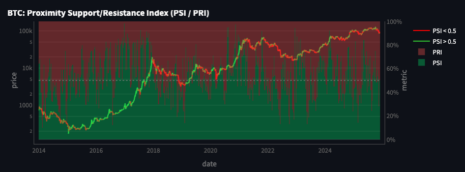
PSR is motivated by a practical observation that also appears repeatedly across on-chain research: the usefulness of cost-basis and positioning signals is highly context-dependent, and often strengthens when the measured cost-basis is close to the current trading range. While the day-to-day shifts in sentiment and realized activity tend to be driven by shorter-horizon holders, when longer-term supply does become responsive, its sheer size can materially influence market outcomes, meaning both short- and long-horizon cost basis can matter, depending on where price is interacting.

This matters more as Bitcoin’s market structure matures. As derivatives markets deepen, they introduce additional synthetic BTC exposure, multiple ways to express demand (or supply) without transacting in the underlying tokens. The result is a larger surface area of “paper” claims that can absorb flows and redistribute positioning, diluting the impact of marginal spot demand and making sustained trends more likely to unfold as extended, two-sided auctions rather than clean, single-direction “blow-off” moves. We’ve already seen this in the current cycle since 2023, with longer consolidations embedded within uptrends compared with earlier, faster bull phases.

In that environment, spot can spend more time oscillating around multiple economically relevant cost basis, increasing the chance that both short-term and long-term supply clusters are simultaneously in play. PSR is designed for exactly this setting: it retains the distributional context but concentrates the signal on the supply most likely to transact at the margin, the supply positioned closest to spot.

Extending to Proximity Market Metrics

PSR's proximity-weighting logic extends naturally into a family of valuation-style metrics. The core building block is the Proximity Realized Price, a weighted average of realized prices across cost-basis quantiles, where cost basis closer to spot carries more weight than cost basis further away. This produces a single, time-varying reference level that reflects the supply most likely to be economically relevant right now, rather than the market's full historical average.

Using this proximity realized price, we can restate two familiar valuation metrics, MVRV and NUPL, on a proximity-weighted basis, so each captures spot price relative to the cost basis nearest to it rather than the market-wide average. We also introduce a third measure, Proximity Premium, which expresses the same spot-to-cost-basis gap in volatility-adjusted terms, making mispricing comparable across different price levels and market regimes.

Proximity MVRV (pMVRV):

$$\text{pMVRV}_t = \frac{P_t}{RP^{\text{proxy}}_t}$$

Proximity NUPL (pNUPL):

$$\text{pNUPL}_t = \frac{P_t - RP^{\text{proxy}}_t}{P_t}$$

Proximity Premium (PP):

• $P_t$ = spot price at time $t$,
• $\sigma^{P}_{30,t}$ = 30-day rolling standard deviation of price,
• $RP^{\text{proxy}}_t$ = proximity realized price at time $t$:

where $RP_{(\varphi,t)}$ is the realized price of cost-basis quantile $\varphi$ at time $t$, and $w_{(\varphi,t)}$ is the weight for quantile $\varphi$ at time $t$, decaying with distance from spot:

$$w_{(\varphi,t)} = \exp\left( -\frac{\lvert P_t - RP_{(\varphi,t)} \rvert}{\sigma^{P}_{30,t}} \right)$$

Conceptually, these measures answer the same questions as their traditional counterparts, valuation vs. cost basis and embedded P/L, but they do so using the part of the cost-basis structure the market is most likely to interact with next.

Reading the Proximity Signals

Proximity-based metrics are designed to be actionable: they retain the intuition of cost-basis positioning but compress it into time series that can be monitored, thresholded, and combined with other signals. Below are a few examples.

Finding Returning Support Before the Rally

From late July to mid-September 2023, BTC drifted down from around 29k to 26k, and PSI sat mostly below 50%, indicating resistance dominance, with more nearby supply positioned above spot than below it. That changed in October: PSI shifted and stabilized above 50%, turning support-dominant. This preceded a sustained push higher, with price climbing from the mid-20Ks into the low 40Ks by December.

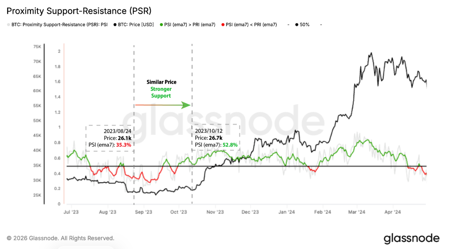
The figure above highlights this shift: on August 24, BTC was at 26.1k with PSI (ema7) at 35.3%; by October 12, price had barely moved to 26.7k, but PSI (ema7) had climbed to 52.8%. Price action over those seven weeks was largely flat, while the underlying support structure shifted meaningfully beneath it.

A similar dynamic played out from February to April 2025. PSI moved from deep resistance dominance in February toward progressively lighter resistance dominance through March, before turning support-dominant in April. This shift preceded another leg higher in price, which climbed from the low-$80Ks toward 120k by midsummer.

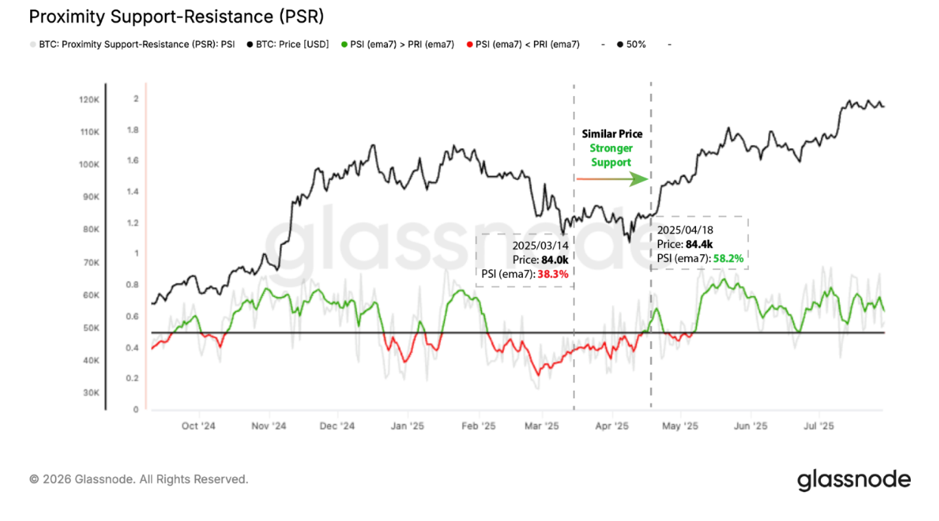
The figure above shows that despite BTC trading at a similar level in mid-March and mid-April, PSI (ema7) moved from high-30%s to high-50%s over that month. This points to accumulation taking place in the intervening weeks, building a stronger support base beneath a price level that otherwise looked unchanged.

Finding Increasing Resistance Before the Drop

The inverse holds as well and can be seen clearly in the two most significant drops of 2026.

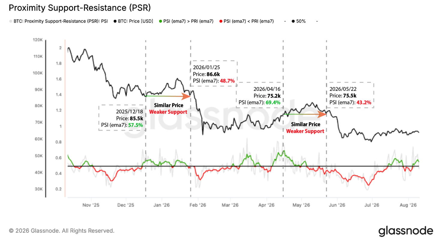
The first came in late 2025 into January 2026. BTC revisited a similar price level twice within about six weeks, at 85.5k on December 18 and 86.6k on January 25, but PSI (ema7) fell from 57.5% to 48.7% over that span, tipping from support-dominant to resistance-dominant. Shortly after, price broke down sharply, falling from the high-$80Ks toward 65k.

The second followed a similar path a few months later, though this time price was climbing higher even as PSI deteriorated underneath it. BTC returned to roughly the same level in mid-April and late May, but PSI (ema7) collapsed from high-60%s to low-40%s in between. This more pronounced shift was due to a strong resistance band between 83.6k and 85.4k that had built up above spot, weighing on the nearby cost-basis structure as price pushed back into that range, leading to the drop into the low-60Ks.

In both cases, price sitting at a familiar level masked a meaningful deterioration underneath it: supply that had been acting as support was increasingly sold into the retest, tipping the balance toward resistance and setting up the subsequent decline.

Reading Exhaustion and Capitulation Cross Cycles

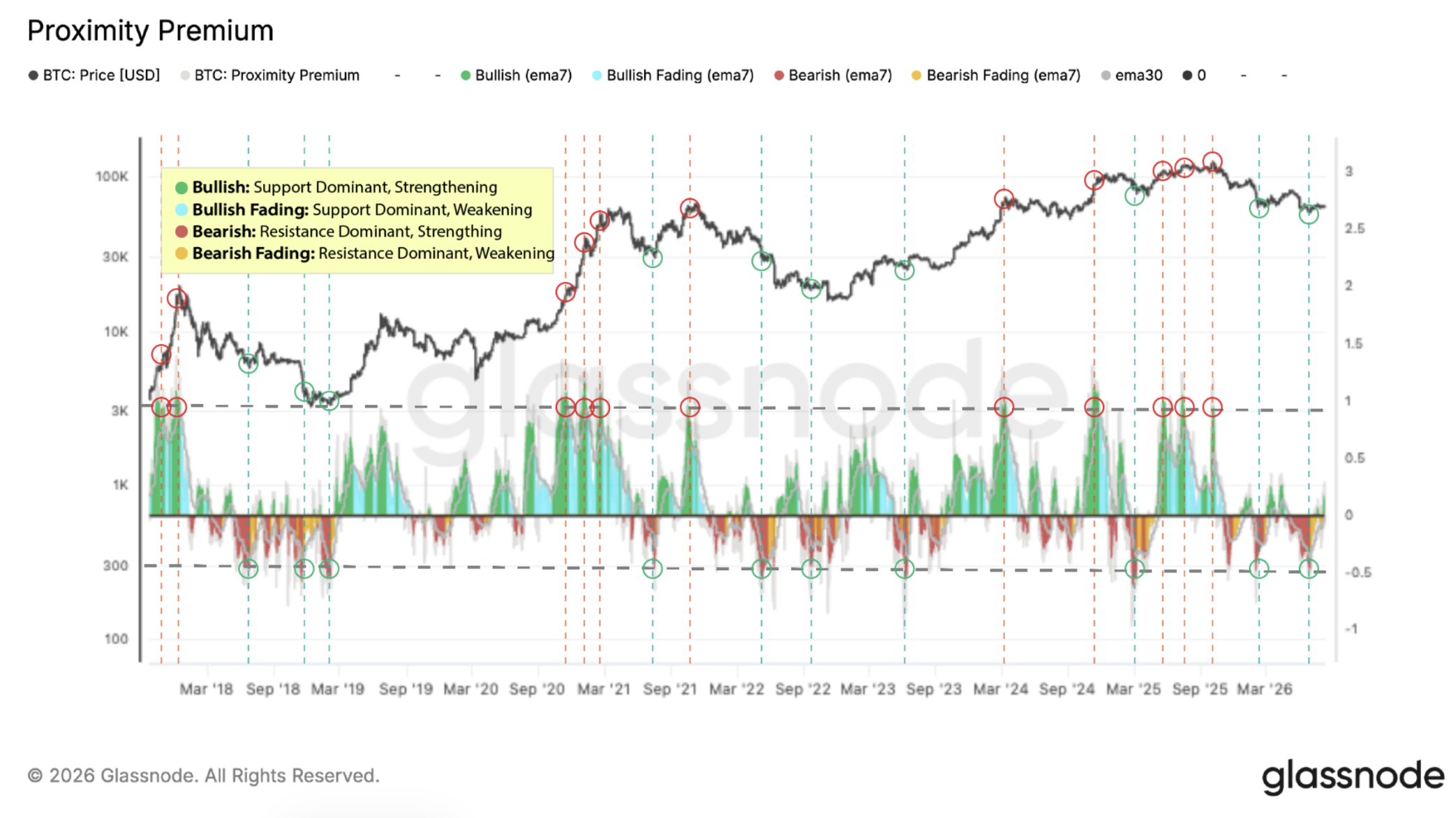
This same logic extends to Proximity Premium, and one useful way to see it in practice is across full market cycles rather than a single episode. Because PP normalizes the spot-to-proximity-cost-basis gap by price volatility, it expresses mispricing in "vol units", making extremes comparable across periods with very different absolute price levels and volatility regimes.

In the figure below, high PP readings (marked in red circles) tend to coincide with locally stretched conditions, where spot has moved far above the proximity cost basis relative to recent volatility, consistent with exhaustion near local and cycle tops. Low PP readings (marked in green circles) tend to mark the opposite: spot falling meaningfully below the proximity cost basis in volatility-adjusted terms, often aligning with sell-pressure climaxes or late-stage capitulation near lows.

Predictive Value of Proximity-Based Cost-Basis Metrics

Beyond these historical examples, it's worth asking whether proximity-based metrics carry predictive value beyond price alone. To test this, we ran a series of regressions for BTC and ETH across multiple forward-return horizons, linking forward returns to lagged price momentum and one on-chain metric at a time, Proximity MVRV, Proximity Premium, or a traditional short-term holder metric like STH-MVRV. At each horizon, we compared how much explanatory power that metric added on top of a baseline model built from past returns alone. The question is straightforward: does adding the on-chain metric meaningfully improve the model's explanatory power, beyond what recent price action already captures?

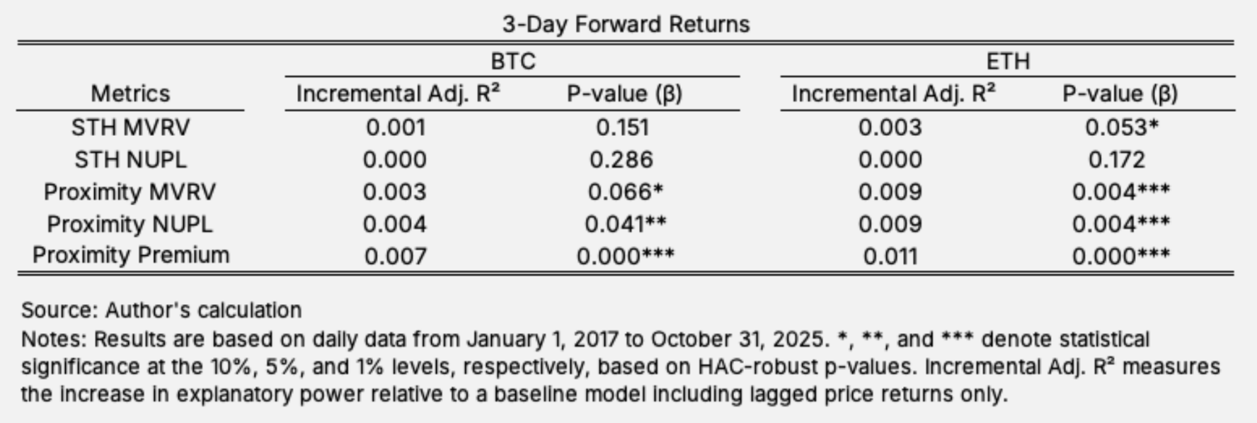
Across all horizons and both assets, proximity-based metrics consistently deliver larger and more statistically robust increases in explanatory power than short-term holder-based aggregates. Proximity Premium stands out in particular, significant at the 1% level for both BTC and ETH, suggesting that where cost basis sits relative to spot carries information about future return regimes that cohort-based measures alone dont capture.

Conclusion

Proximity-weighted cost-basis metrics provide a practical way to translate cost-basis distributions into clean, interpretable time series. PSR (via PSI/PRI) summarizes how near-price cost basis is positioned relative to spot, while proximity realized price enables proximity-based versions of familiar valuation measures such as pMVRV, pNUPL, and the volatility-normalized Proximity Premium.

These proximity signals focus on the supply most likely to transact next, not the supply that merely dominates the historical average. In the predictive tests, they also appear to contain forward-looking information about return regimes beyond what is captured by recent price dynamics, and they outperform common short-term holder aggregates on an incremental explanatory basis. For practitioners, this means a more actionable, near-price view of positioning, one that can help frame whether rallies are likely to be absorbed by overhead supply, whether pullbacks are likely to find nearby support, and when volatility-adjusted dislocations are reaching historically meaningful extremes.

This is an article from Vicky Yang, co-founder at Fountainhead Digital.